The intention of project is to transform and utilize the Ames Housing Dataset to understand how different property features affect Sale Price.
You can find the source code and project files on GitHub:
View GitHub RepositoryThe Ames Housing dataset contains 2930 observations of sold residential properties from 2006 - 2010. (Ames, IA)
Data Structure
- 82 variables
- Sale Price as Dependent Variable
- See All Variables Here
To anchor this project, we can make the following assumption using domain knowledge:
- Property Size: Larger properties will likely command higher sale prices.
- Neighborhood: Properties located in premium neighborhoods will be priced higher due to demand and amenities.
- Overall Quality: Building material quality and property condition will play a significant role in determining the price.
- Year Built: Newly constructed or recently renovated properties will tend to have higher prices compared to older ones.
- Garage Size: Larger garages may increase a property's value due to added utility.
This can be translated into the following Null Hypotheses:
- H₀ = Property size is not a significant predictor of price.
- H₀ = Neighborhood is not a significant predictor of price.
- H₀ = Overall quality is not a significant predictor of price
- H₀ = Age of property is not a significant predictor of price.
- H₀ = Garage capacity is not a significant predictor of price
Data Treatment & Cleaning
1. Calculating Growth Rate Using Median Sale Price (2006–2024)
The growth rate of property values was calculated using the compound annual growth rate (CAGR) formula:
- CAGR = (Median Sale Price (2024) / Median Sale Price (2006))^(1 / Years) - 1
2. Compounding Sale Price Using Growth Rate
Using the calculated growth rate, the future value of sale prices was forecasted using the formula:
- Future Value = Current Sale Price × (1 + Growth Rate)^Years
3. Cleaning Data
-
Imputing Missing Values:
Missing values were treated as follows, based on validation using other variables in the dataset:
- Numerical features (e.g., GarageArea, BsmtFinSF1) were filled with 0 when the absence of a feature (e.g., no garage or no basement) was confirmed.
- Categorical features (e.g., PoolQC, MiscFeature) were filled with None when the missing values represented the absence of that feature (e.g., no pool or no shed).
- For features dependent on neighborhoods (e.g., LotFrontage), missing values were imputed with the median value of the neighborhood to account for local variation.
-
Feature Engineering:
Three variables were engineered:
- TotalSQFT: Sum of GrLivArea and TotalBsmtSF.
- Decade Built: Calculated as the floor division of Year Built by 10, multiplied by 10
- TotalBaths: Sum of full and half bathrooms, including basement bathrooms:
- FullBath + (0.5 × HalfBath) + BsmtFullBath + (0.5 × BsmtHalfBath)
4. Encoding Features
- Nominal Features: One-hot encoding was applied using pd.get_dummies to handle variables such as Neighborhood and Exterior1st.
-
Ordinal Features: Custom mappings were applied to features like ExterQual and
KitchenQual to encode their ordinal nature:
- ExterQual Mapping: Excellent (5), Good (4), Average (3), Fair (2), Poor (1).
Understanding the Dataset
To gain a contextual understanding of the dataset and sale price, let's first compare the summary statistics of the original sale price and the adjusted sale price.
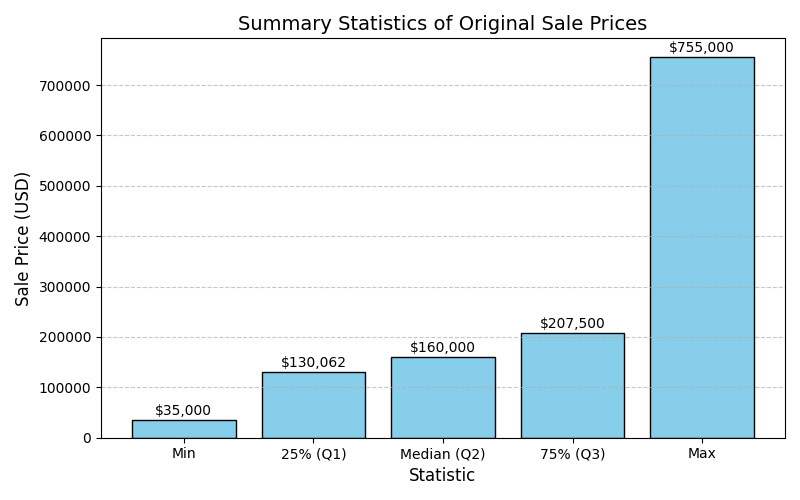

Observing these two charts, we can identify significant outliers on both end of the spectrum. However, the typical price of properties often range between 130-200k for the orignal sale price and 200-300k for the adjusted sale price.
Just gleaning from this information we can make an assumption that Ames properties would fall in the category of affordable housing. Just as a note, moving forward any sale price will be referring to the adjusted sale price.
Let's also visualize the distribution of the sale price to see if we can glean any additional insights:
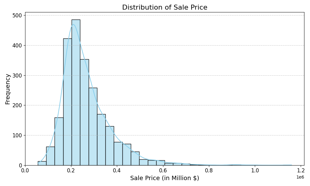
Based on the distribution curve, we can observe:
- A majority of the properties have sale prices concentrated in the lower to mid-price range.
- A right skew; indicating outliers of high-value properties that exceed the typical price range.
- The mode appears to be around the $200,000 - $250,000 region; suggesting this is the most common range for property sale prices.
- An outlier property reached a sale value of $1.2 million; although such cases are scarce.
Now let's visualize the relationship between TotalSQFT and Sale Price:
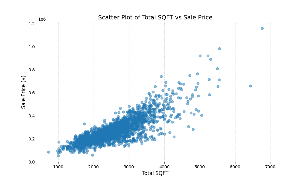
Based on the scatter plot above, we can observe:
- A positive correlation; there is a clear positive trend where an increase in total square footage generally correlates with a high sale price. Though, it is important to note that there is some variability.
- The data points are densely clustered around smaller property sizes (1,000–3,000 SQFT) and lower sale prices ($100,000–$400,000). This reflects the most common property size and price range in the dataset.
- For properties below 3,000 SQFT, the relationship between size and price is tighter and more consistent, while larger properties show greater variability in sale prices, likely influenced by other variables.
- Although this chart alone is not sufficient evidence, it does suggest rejecting the null hypothesis that property size does not affect sale price.
- We will validate its significance later when we conduct our regression analysis.
Next, let's take a look at the relationship between neighborhoods and sale price:
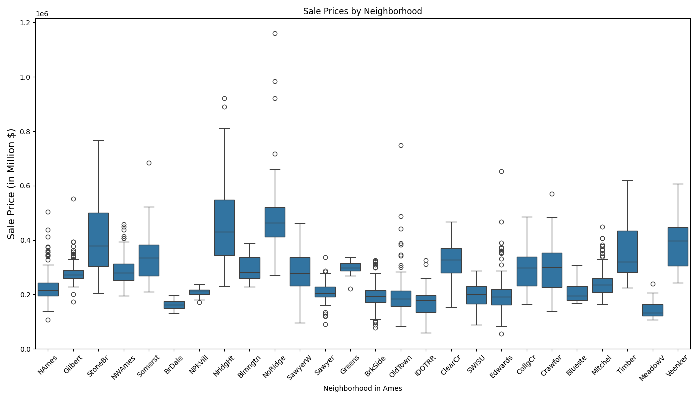
Based on the boxplot above, we can observe:
- Variation in sale price varies across different neighborhoods.
- Neighborhoods like StoneBr (Stone Brook), NridgHt (Northridge Heights), and NoRidge (Northridge) have higher median sale prices, indicating they are luxury or high-value areas.
- Whereas Neighborhoods like MeadowV (Meadow Village), BrDale (Briardale), and Edwards have lower median sale prices, suggesting affordability.
- Wide IQRs (e.g., NridgHt, NoRidge) suggest high variability in sale prices, likely due to diverse property features.
- Narrow IQRs (e.g., BrDale, MeadowV) indicate uniform property values within those neighborhoods.
- The box plot suggests rejecting the null hypothesis (H₀), as neighborhood significantly impacts sale price.
- To verify this suggestion, a one-way ANOVA test was conducted using Neighborhood as the categorical independent variable and Sale Price as the dependent variable.
- The resulting p-value = 0.0 which validates the neighborhood's statistical significance; hence the neighborhood's H₀ can be rejected.
Moving on, let's visualize the relationship between overall quality and sale price:
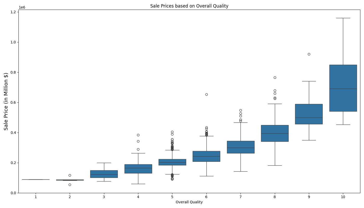
Based on the boxplot above, we can observe:
- A strong positive relationship between quality and sale price
- Properties with Overall Quality = 2 have very low sale prices.
- Properties with Overall Quality = 10 have significantly higher median sale prices.
- As the overall quality improves, the spread (range) of sale prices also increases; likely influenced by other variables.
- There are notable outliers in several quality levels (e.g., 5, 7, 8, and 10), indicating that some properties sell for much higher or lower prices than expected within those categories; potentially indicating that they might belong to different market segments or is inclusive of special features.
- Overall, a one-way ANOVA test confirms Overall Quality's statistical significance with a p-value = 0.0, therefore, reject H₀.
Moving on to Year Built:
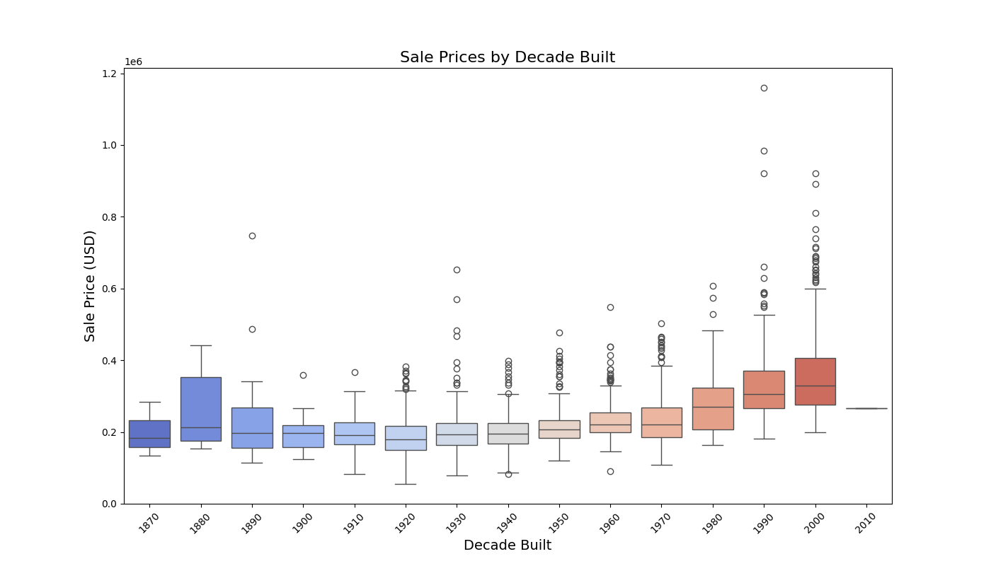
Based on the box plot above, we can observe:
- Sale prices generally increase for properties built in more recent decades, with a noticeable upward trend starting from 1980s onwards.
- Median sale prices for properties built in the 2000s are significantly higher compared to earlier decades; suggesting a preference for recently built properties.
- Older properties (pre-1940) have a narrower range of sale prices, indicating more uniform pricing; with exclusion of 1880, potentially due to recent renovation.
- Variances in outliers begins to a become more pronounced from 1980s onwards as evidenced by the taller boxplots and longer whiskers.
- An ANOVA test confirms our suspicion that Decade Built is a statistically significant predictor of price. Reject H₀.
Lastly, lets visualize the relationship between garage capacity and sale price:
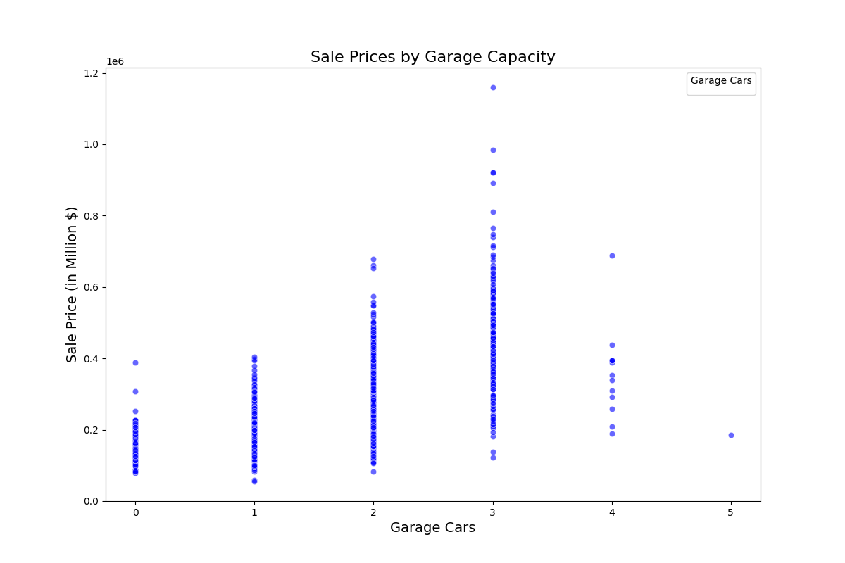
Based on the scatter plot above we can observe:
- There is a positive correlation whereby a higher garage capacity is associated with higher-value properties.
- Properties with no garage are clustered at the lower end of sale prices, indicating that garage space is a salient feature when determining home value
- Most homes have a garage space for between 1-3 cars. With 2 car garages being the most common. However, high-value properties are more associated with 3 car garages
- Interestingly, the price of properties with 4 or 5 car garages begins to slope down, although there are not enough data points in these two categories to infer meaningful insights.
- An ANOVA test confirms that garage capacity are is a significant predictor of price. Therefore, reject H₀.
Data Modeling
The goal of this section is to go beyond simple visualizations and statistical tests to uncover the nuanced relationships between independent variables and the dependent variable (sale price). This dataset includes many correlated variables (e.g., Garage Cond, Garage Area, Garage Cars, Garage Qual), which can introduce multicollinearity in regression models. So first task on the agenda is to handle multi-collinearity.
This is the original numerical variables list:
Lot Frontage      float64
Lot Area          int64
Overall Qual      int64
Overall Cond      int64
Year Built        int64
Year Remod/Add    int64
Mas Vnr Area      float64
BsmtFin SF 1      float64
BsmtFin SF 2      float64
Bsmt Unf SF       float64
Total Bsmt SF     float64
1st Flr SF        int64
2nd Flr SF        int64
Low Qual Fin SF   int64
Gr Liv Area       int64
Bsmt Full Bath    float64
Bsmt Half Bath    float64
Full Bath         int64
Half Bath         int64
Bedroom AbvGr     int64
Kitchen AbvGr     int64
TotRms AbvGrd     int64
Fireplaces        int64
Garage Yr Blt     float64
Garage Cars       float64
Garage Area       float64
Wood Deck SF      int64
Open Porch SF     int64
Enclosed Porch    int64
3Ssn Porch        int64
Screen Porch      int64
Pool Area         int64
Misc Val          int64
Mo Sold           int64
Yr Sold           int64
SalePrice         int64
However, if you recall, we engineered 2 unique variables from their counterparts: TotalSQFT, and TotalBaths. So from these these three variables, we can remove the following variables:
BsmtFin SF 1      float64
BsmtFin SF 2      float64
Bsmt Unf SF       float64
Total Bsmt SF     float64
1st Flr SF        int64
2nd Flr SF        int64
Low Qual Fin SF   int64
Gr Liv Area       int64
Bsmt Full Bath    float64
Bsmt Half Bath    float64
Full Bath         int64
Half Bath         int64
After removal, we are left with:
Bedroom AbvGr     int64
Kitchen AbvGr     int64
TotRms AbvGrd     int64
Fireplaces        int64
Garage Yr Blt     float64
Garage Cars       float64
Garage Area       float64
Wood Deck SF      int64
Open Porch SF     int64
Enclosed Porch    int64
3Ssn Porch        int64
Screen Porch      int64
Pool Area         int64
Misc Val          int64
Mo Sold           int64
Yr Sold           int64
SalePrice         int64
Year Remod/Add    int64
Mas Vnr Area      float64
Lot Frontage      float64
Lot Area          int64
Overall Qual      int64
Overall Cond      int64
Based on the remaining numerical variables, only the following variables are experiencing multi-collinearity (corr > .7). As a solution, we can drop the garage area variable from our variable list.
Now that we've handled multi-collinearity, let's start off with a basic regression model to establish a baseline:
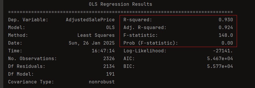
Dependent Variable: The model is designed to predict AdjustedSalePrice
R-squared (0.930): This metric quantifies the proportion of variability in AdjustedSalePrice explained by the predictors in the model. A value of 93% indicates the model provides an excellent fit to the data. However, this high value warrants scrutiny for potential overfitting, especially with a large number of predictors.
Adjusted R-squared (0.924): This adjusted metric accounts for the inclusion of 191 predictors, penalizing the addition of variables that do not significantly improve the model's explanatory power. The minimal difference between R² and Adjusted R² suggests that most predictors contribute meaningful information, though some may still be redundant or insignificant.
F-statistic (148.0) and Prob (F-statistic = 0.00):
- The F-statistic tests the joint null hypothesis that all regression coefficients (excluding the intercept) are zero.
- A high value of 148 and a p-value of 0.00 strongly reject this null hypothesis, indicating that at least one predictor significantly explains variation in AdjustedSalePrice.
- The magnitude of the F-statistic reflects the collective explanatory strength of the model.
Number of Observations (2326): The sample size provides robust statistical power, reducing the likelihood of Type II errors. However, with 191 predictors, the ratio of predictors to observations (approximately 1:12) should be monitored to avoid overparameterization.
Degrees of Freedom (Df):
- Df Residuals (2134): Indicates the number of independent observations remaining after estimating 191 model parameters. A large residual degree of freedom ensures stable parameter estimates.
- Df Model (191): Represents the number of predictors, reflecting the model's complexity. With this many predictors, multicollinearity and overfitting risks must be addressed.
The OLS regression model provides a strong explanation of the variability in AdjustedSalePrice, with an R^2 of 93% and an adjusted R^2 of 92.4%, indicating excellent predictive power while accounting for the large number of predictors. The model is statistically significant overall, as evidenced by an F-statistic of 148 and a corresponding p-value of 0.00, which strongly rejects the null hypothesis that all predictors have no effect on AdjustedSalePrice. However, the complexity of the model, with 191 predictors and a predictor-to-observation ratio of approximately 1:12, warrants careful evaluation of multi-collinearity and overfitting.
To refine this model, let's build the model again, this time removing insignificant (variables with p-value < .05)
Based on the result of the initial regression model, the following variables has a p-value of < 0.05 (and will therefore, be dropped):
Lot Shape
Utilities
Land Slope
Year Remod/Add
Exter Cond
Bsmt Cond
BsmtFin Type 2
Electrical
Kitchen AbvGr
Fireplace Qu
Garage Yr Built
Garage Finish
Garage Qual
Garage Cond
Paved Drive
Open Porch SF
Enclosed Porch
3Ssn Porch
Fence
Misc Val
Mo Sold
MS Zoning
Street
Alley
Roof Style
Heating
Misc Feature
After dropping the insignificant variables and re-running model again, this is the result:

After removing the redundant variables, the predictive power of the model remains largely unaffected, as evidenced by the negligible difference between the R^2 and Adjusted R^2 . This demonstrates that the excluded variables contributed little to explaining the variance in the dependent variable, reaffirming the validity of the remaining predictors. Additionally, the reduction in the number of parameters from 191 to 150 has significantly simplified the model, improving its interpretability and reducing the risk of overfitting. By focusing only on the most meaningful variables, the model strikes a balance between simplicity and statistical robustness, ensuring it remains both computationally efficient and generalizable to new data.
While reducing the model parameters to 150 is a step in the right direction, it is still relatively high for practical use, particularly if the goal is to serialize the model for deployment in real-world applications, such as predicting property prices using Zillow data. A simpler, more parsimonious model would streamline predictions and ensure ease of implementation in systems with limited computational resources. However, this simplification often comes with a trade-off—sacrificing some predictive power for practicality. Therefore, it is crucial to evaluate priorities: whether to prioritize a complex yet highly accurate model or a more practical, lightweight model that balances efficiency and usability.
My next step in simplifying the model involves removing all categorical variables from the regression. Based on my observations, the majority of categorical variables are statistically insignificant, with only a few showing meaningful relationships with the dependent variable. Retaining these variables adds unnecessary complexity without substantially improving the model's predictive power. By excluding them, the model can focus solely on the numerical predictors that are more relevant and impactful, further simplifying its structure while maintaining its validity for practical applications. This approach will also streamline model serialization and deployment for real-world use cases, such as property price prediction.
After dropping all categorical variables, and insignificant numerical variables this is the result of the regression:
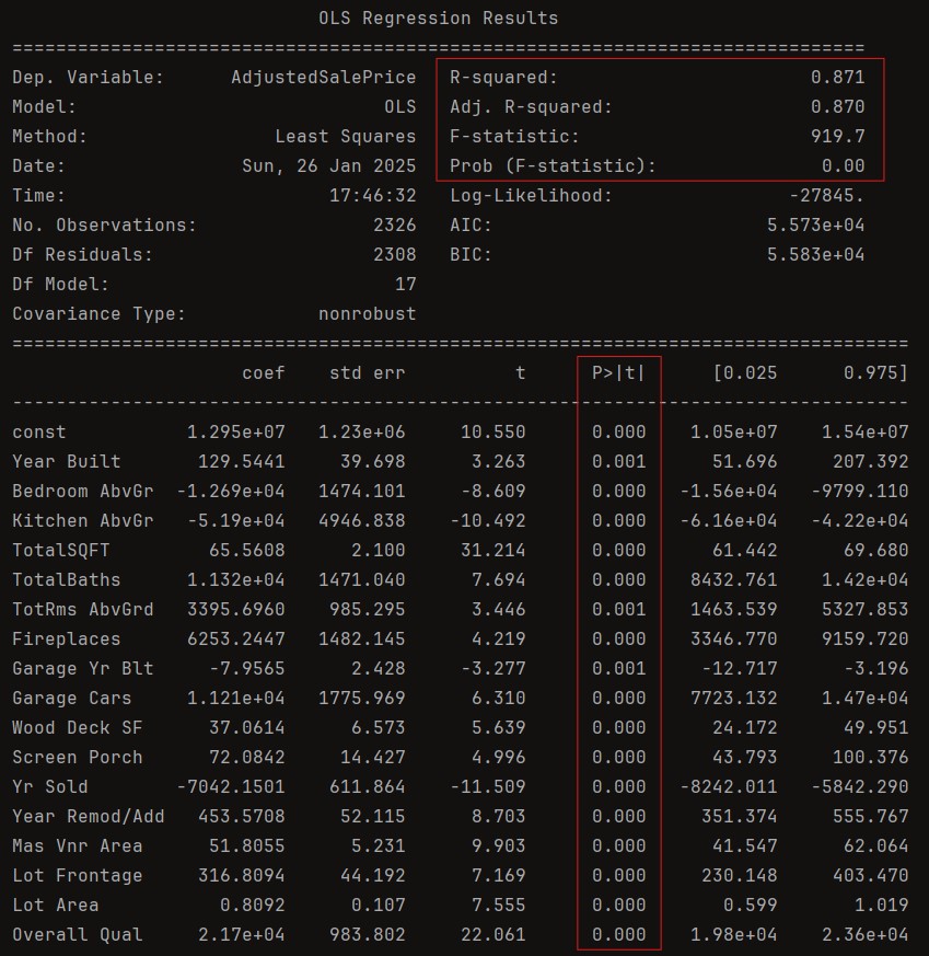
We successfully reduced number of predictors from 191 to just 17, significantly simplifying its structure. The R^2 value is now 87.1%, with an Adjusted R^2 of 87%, indicating a slight reduction in predictive power. However, considering the drastic reduction in complexity, this sacrifice is relatively minor and well worth the improved practicality. This streamlined model is far more suitable for real-world applications, such as predicting property prices. The next step is to assess whether these remaining predictors correspond to information readily available for properties listed on Zillow, ensuring the model's feasibility for deployment.
Using this zillow listing as an example, the following table highlights how the property details from Zillow are mapped to the regression model variables:
| Model Variable | Zillow Information | Notes |
|---|---|---|
| Year Built | 1975 | Directly listed in Zillow. |
| Bedroom AbvGr | 3 | Listed under Bedrooms. |
| Kitchen AbvGr | 1 | Assumed to be 1 based on data. |
| TotalSQFT | 2,050 sqft | Sum of above and below ground living areas. |
| TotalBaths | 2.0 | Calculated from full and 3/4 bathrooms. |
| TotRms AbvGrd | 6 | Counted based on listed main-level rooms. |
| Fireplaces | 0 | Assumed absent as not mentioned. |
| Garage Yr Blt | 1975 | Assumed to match Year Built. |
| Garage Cars | 1 | Assumed based on garage presence. |
| Wood Deck SF | Unknown | Listed as a feature but no size provided. |
| Screen Porch | 0 | Assumed absent as not mentioned. |
| Yr Sold | 2025 | Based on listing year. |
| Year Remod/Add | 1975 | Assumed no remodeling occurred. |
| Mas Vnr Area | 0 | Assumed no masonry veneer. |
| Lot Frontage | Unknown | Not listed; may need estimation. |
| Lot Area | 10,018 sqft | Directly listed in Zillow. |
| Overall Qual | Unknown | Subjective; requires estimation. |
Based on the mapping above, it appears that only Lot Frontage and Wood Deck SF should be considered for removal, as it lacks a clear assumption or direct mapping from available property data (e.g., Zillow). While it can be imputed with a median value to retain consistency in the dataset, doing so might introduce noise or reduce model interpretability. Instead, excluding Lot Frontage and Wood Deck SF simplifies the model further while only sacrificing a small amount of predictive power (reduced R^2 by .004), ensuring that the model remains practical and easy to deploy with real-world property data.
Now that we've decided on the significant predictors of properties, let's experiment with various predictive models, to see which yields the highest R^2 before we serialize the model.
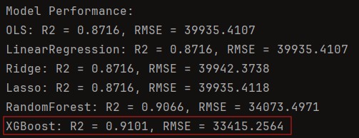
Given that XGBoost outperformed other models, the next step is to serialize the XGBoost model using joblib. Once serialized, we can turn it into an API that allows you to input property details, such as those from Zillow, and predict property prices seamlessly. This approach ensures that the model is both portable and easily deployable for real-world use.
But what if we wanted to really ask—what makes this process worth our time? What value can we truly extract from this dataset?
Despite the challenges of predicting current property prices due to limited data, this dataset offers invaluable insights into property valuation. By examining key features, we can form a practical, value-oriented strategy for identifying properties with strong investment potential.
Here's how each variable contributes to the story:
- Bedrooms Above Ground, Kitchens Above Ground, Total Rooms Above Ground: These variables provide insight into a home's livable space. More rooms, especially in well-designed layouts, often attract higher sale prices due to greater functional appeal for families.
- Fireplaces: Fireplaces add a traditional and aesthetic value to properties. Homes with this feature can stand out in the market, particularly in colder climates.
- Garage (Year Built, Car Capacity, Area): The presence and quality of a garage significantly impact the property's value. Larger garages with multiple car capacity are appealing in suburban and high-income areas where vehicle ownership is common.
- Wood Deck SF, Open Porch SF, Enclosed Porch, 3-Season Porch, Screen Porch: Outdoor living spaces, such as decks and porches, contribute to a property's recreational appeal. Well-maintained outdoor areas often increase buyer interest and perceived home value.
- Pool Area: Pools are luxury features that can substantially increase property value in warm climates but might not add as much value in colder regions where maintenance costs deter potential buyers.
- Miscellaneous Value: This represents other unique property features, such as sheds, fences, or custom landscaping, which may influence sale price depending on buyer priorities.
- Month Sold, Year Sold: Seasonality plays a key role in real estate markets. Properties sold during peak seasons (e.g., spring and summer) tend to fetch higher prices due to increased demand.
- Year Remodeled/Added: Recent renovations increase property appeal and marketability. Modern upgrades often translate into higher sale prices, particularly for older homes.
- Lot Frontage and Lot Area: The size and frontage of a property affect both development potential and perceived spaciousness. Larger lots typically command higher prices, especially in desirable neighborhoods.
- Overall Quality and Condition: These comprehensive measures assess a home's construction quality and current state. Properties with high-quality materials and excellent maintenance are more likely to sell at a premium.
By using these variables, investors and real estate professionals can create a structured approach to property selection. For instance, homes with favorable combinations of large lot sizes, recent renovations, and multiple amenities—such as garages and porches—are statistically likely to offer better resale value. This allows us to strategically prioritize which properties to renovate, acquire, or flip for maximum profitability.
Although precise predictions remain challenging due to dataset limitations, the ability to extract meaningful patterns from these variables helps guide informed decision-making in real estate investment, making this data analysis a valuable tool.
Limitations of Domain Knowledge in Implementation
While identifying statistically relevant features is crucial, the effective application of this information requires domain-specific knowledge. Real estate markets vary widely across regions, and the significance of certain features can differ depending on local buyer preferences, economic conditions, and regulatory factors. For instance, the value added by a pool or outdoor living area may be substantial in warmer climates but negligible in colder areas where these features are rarely used.
Additionally, factors such as zoning laws, school districts, and proximity to amenities are not captured within this dataset but are often critical to a property's value. Without an understanding of these domain-specific influences, our analysis risks misinterpreting or oversimplifying the data's implications.
Therefore, the key takeaway is that data analysis alone is not enough; success depends on combining statistical insights with expert knowledge of the real estate market. By marrying these two perspectives, investors can make better-informed decisions, minimizing risk and maximizing the potential for high returns.